Layering Data
Monday, January 21, 2013
Layering is defined as the action of arranging something into layers. There are various reasons to why data is layered but I think the most important one is to show a more accurate picture about something. Each layer may contain different information so when the layers are combined all of the information can be seen. Providing a more accurate picture about something even applies in Digital Forensics and Incident Response (DFIR). I saw its benefits when layering different artifacts showing similar information such as the installed software artifacts. A single artifact may not show all of the software that is or was installed but looking at the information from all artifacts provide a more accurate picture of what programs were on a computer. I have found layering data to be a powerful technique; from what programs executed to what files were accessed to what activity occurred on a system. I hope to demonstrate the benefits to layering data through the eye of a timeline.
Before diving into timelines I wanted to take a step back to first illustrate layering data. The best visual example of how layering data provides a more accurate picture of something is the way mapping software works. All layers contain information about the same geographical location but the data each layer contains is different.
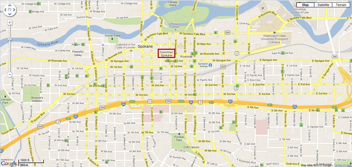
I wanted to use an example closer to home to show the additional information layering data in maps provides. When my wife and I were looking for a house to buy one of the things we took into consideration was the crime rate in the neighborhood. We didn’t want to end up in a rough neighborhood so we wanted additional information about the neighborhoods we were looking at. Unfortunately, there are no online crime maps where I live so I had to settle for the City of Spokane, Washington Crime Map I found with a Google search. Let’s say my wife and I were looking at a loft in downtown Spokane located in the red box on the map.

Using the crime map I first wanted to know what burglaries occurred over the past month.

So far so good; there were a few burglaries that occurred but none were inside the red box. A month doesn’t provide an accurate picture; let’s see the statistics for the past year.

Adding this additional layer provides more information about the burglaries in the area. Like most people, we are more worried about all crime as opposed to just one type of crime. Adding the all crime layer to the map provides even more information.

The new layer provides more information about the crime in the downtown area but adding another layer will provide more even more context. I added the heat map layer as shown below.

The heat map layer now shows an accurate picture about the crime rate around downtown Spokane where our imaginary loft is located. The loft is located in the area that has the highest concentration of crime. By layering data on top of the geographic location we were interested in would enable us to make a more informed decision about if we would actually want to live there. Please note: I only used Spokane since it was the first crime map I saw on a Google search. I have no knowledge about the downtown area and it might be a great place to live.
System timelines are a great way to illustrate layering data in DFIR. Artifacts can be organized into layers and then applied to a timeline as a group. The easiest way to see this is by looking at the examination process I use. Below are a few of my examination steps:
- Examine the programs ran on the system
- Examine the auto-start locations
- Examine the host-based logs
- Examine file system artifacts
I tend to group artifacts together underneath the examination step they pertain to. In other words, I organize all artifacts based on categories that match my examination step. For example, the files listed underneath the examine file system artifacts step include: $MFT, $LogFile, $UsnJrnl, and $INDX files. When I want to know something about the file system then I will examine all of these artifacts. I discussed this examination approach before when I wrote about how to obtain information about the operating system (side note: I updated the script and it automates my entire registry examination process). Harlan shared his thoughts about the usefulness of categorizing artifacts in his post There Are Four Lights: The Analysis Matrix. SANs released their DFIR poster which organizes artifacts based on categories. In my opionion this is the best technqiue when approahing an examination and to deomonstrate it I’ll use the image from the post Extracting ZeroAccess from NTFS Extended Attributes.
In the post I mentioned how ZeroAccess modified the services.exe file so it loads the Trojan from the NTFS Extended Attributes. I parsed the $MFT with AnalyzeMFT. The services.exe file was timestomped using file system tunneling; I focused on the timestamp for the last MFT update which was 12/06/2012 22:18:06.

The $MFT by itself provides a wealth of information but it doesn’t provide any historical information. This is where layering data comes into play and the other NTFS artifacts. I parsed the $LogFile with David Cowen’s Advanced NTFS Journal Parser public version and added it to the timeline (check out his other post Happy new year, new post The NTFS Forensic Triforce to see how the NTFS artifacts tie together).

The $Logfile provided a little more context about the time when the services.exe $MFT record was last updated. The rows in blue shows a file was renamed followed by services.exe being created. Let’s continue layering data by adding the information stored in the $UsnJrnl file. I parsed the file with Tzwork’s Windows Journal Parser and added it to the timeline.

The $UsnJrnl also shows the services.exe file was renamed before it was created as well as other changes made to the file’s attributes.
The timeline only contained one layer of artifacts which were the NTFS artifacts. Combining the information stored in the $MFT, $LogFile, and $UsnJrnl provided more context about the services.exe file and how it came to be. Even more information could be obtained by adding more layers to the timeline such as program execution and logging information. Layering data in DFIR should not be limited to timelines. Every artifact can be organized into categories and the categories themselves can be treated as layers of information.
Layering Data in Action
Before diving into timelines I wanted to take a step back to first illustrate layering data. The best visual example of how layering data provides a more accurate picture of something is the way mapping software works. All layers contain information about the same geographical location but the data each layer contains is different.
I wanted to use an example closer to home to show the additional information layering data in maps provides. When my wife and I were looking for a house to buy one of the things we took into consideration was the crime rate in the neighborhood. We didn’t want to end up in a rough neighborhood so we wanted additional information about the neighborhoods we were looking at. Unfortunately, there are no online crime maps where I live so I had to settle for the City of Spokane, Washington Crime Map I found with a Google search. Let’s say my wife and I were looking at a loft in downtown Spokane located in the red box on the map.

Using the crime map I first wanted to know what burglaries occurred over the past month.
So far so good; there were a few burglaries that occurred but none were inside the red box. A month doesn’t provide an accurate picture; let’s see the statistics for the past year.

Adding this additional layer provides more information about the burglaries in the area. Like most people, we are more worried about all crime as opposed to just one type of crime. Adding the all crime layer to the map provides even more information.

The new layer provides more information about the crime in the downtown area but adding another layer will provide more even more context. I added the heat map layer as shown below.

The heat map layer now shows an accurate picture about the crime rate around downtown Spokane where our imaginary loft is located. The loft is located in the area that has the highest concentration of crime. By layering data on top of the geographic location we were interested in would enable us to make a more informed decision about if we would actually want to live there. Please note: I only used Spokane since it was the first crime map I saw on a Google search. I have no knowledge about the downtown area and it might be a great place to live.
Layering Data in Timelines
System timelines are a great way to illustrate layering data in DFIR. Artifacts can be organized into layers and then applied to a timeline as a group. The easiest way to see this is by looking at the examination process I use. Below are a few of my examination steps:
- Examine the programs ran on the system
- Examine the auto-start locations
- Examine the host-based logs
- Examine file system artifacts
I tend to group artifacts together underneath the examination step they pertain to. In other words, I organize all artifacts based on categories that match my examination step. For example, the files listed underneath the examine file system artifacts step include: $MFT, $LogFile, $UsnJrnl, and $INDX files. When I want to know something about the file system then I will examine all of these artifacts. I discussed this examination approach before when I wrote about how to obtain information about the operating system (side note: I updated the script and it automates my entire registry examination process). Harlan shared his thoughts about the usefulness of categorizing artifacts in his post There Are Four Lights: The Analysis Matrix. SANs released their DFIR poster which organizes artifacts based on categories. In my opionion this is the best technqiue when approahing an examination and to deomonstrate it I’ll use the image from the post Extracting ZeroAccess from NTFS Extended Attributes.
In the post I mentioned how ZeroAccess modified the services.exe file so it loads the Trojan from the NTFS Extended Attributes. I parsed the $MFT with AnalyzeMFT. The services.exe file was timestomped using file system tunneling; I focused on the timestamp for the last MFT update which was 12/06/2012 22:18:06.
The $MFT by itself provides a wealth of information but it doesn’t provide any historical information. This is where layering data comes into play and the other NTFS artifacts. I parsed the $LogFile with David Cowen’s Advanced NTFS Journal Parser public version and added it to the timeline (check out his other post Happy new year, new post The NTFS Forensic Triforce to see how the NTFS artifacts tie together).

The $Logfile provided a little more context about the time when the services.exe $MFT record was last updated. The rows in blue shows a file was renamed followed by services.exe being created. Let’s continue layering data by adding the information stored in the $UsnJrnl file. I parsed the file with Tzwork’s Windows Journal Parser and added it to the timeline.

The $UsnJrnl also shows the services.exe file was renamed before it was created as well as other changes made to the file’s attributes.
Summary
The timeline only contained one layer of artifacts which were the NTFS artifacts. Combining the information stored in the $MFT, $LogFile, and $UsnJrnl provided more context about the services.exe file and how it came to be. Even more information could be obtained by adding more layers to the timeline such as program execution and logging information. Layering data in DFIR should not be limited to timelines. Every artifact can be organized into categories and the categories themselves can be treated as layers of information.
Labels:
categories,
NTFS,
timeline


Great stuff, Corey, thanks for sharing!
Great post, great information. I am struggling with the difference between the $logfile and $usnjrnl arctifacts...They seem to contain similar type of information,i just don't get why an artifact would be in one vs the other. Any light you could share on that would be appreciated.
@Kx499
I agree some information recorded in the $LogFile and $UsnJrnl is similar. Both record actions taking against a file such as creation, deletion, and renaming. However, there are some notable differences such as the $LogFile logs timestamps. To get a better idea about the differences between these files I would read David's posts:
http://hackingexposedcomputerforensicsblog.blogspot.com/2013/01/happy-new-year-new-post-ntfs-forensic.html
then
http://hackingexposedcomputerforensicsblog.blogspot.com/2013/01/ntfs-triforce-deeper-look-inside.html
One thing to keep in mind is that $UsnJrnl didn't start being used by default until Vista. I have never seen a $UsnJrnl file on a XP machine while I have seen $LogFile on both XP, Vista, and 7.